Support Vector Machine (SVM)
1. Introduction to problem to be solved
In many machine learning problems, the objective is to separate different groups of data.
For example, we may want to distinguish between cats and dogs, approved and rejected loan applications, or spam and legitimate emails.
The goal is to find a decision boundary that separates one class from another.
As illustrated in the figure below:
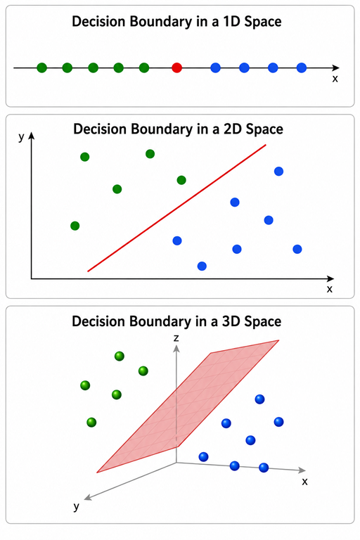 |
- In a 1D feature space, the decision boundary is a point. - In a 2D feature space, the decision boundary is a line. - In a 3D feature space, the decision boundary is a plane. The same idea extends naturally to higher-dimensional feature spaces, where the decision boundary becomes a hyperplane. |
Support Vector Machine (SVM) is one of the machine learning algorithms that solves this problem. It searches for a decision boundary that best separates different classes of data.
2. What is SVM
-
Support Vector Machine (SVM) is a supervised machine learning algorithm used for:
- Classification
- Regression (predicting continuous values)
SVM is like drawing the best possible dividing boundary between two groups of data.
(Although SVM can also be used for regression (called Support Vector Regression, or SVR), this article focuses on classification.)
3. A simple example
-
Suppose we want a machine to identify:
1. cat 2. dog -
We give it 2 parameters (features) only:
1. weight
2. size
Step 1: Create dataset
| Animal | Weight (kg) | Size (cm) |
|---|---|---|
| Cat | 4 | 25 |
| Cat | 5 | 28 |
| Cat | 6 | 30 |
| Dog | 18 | 60 |
| Dog | 22 | 70 |
| Dog | 25 | 75 |
Step 2: Plot the points
-
Imagine a graph:
x-axis = weight y-axis = size -
Cats appear clustered in one area:
smaller lighter -
Dogs appear in another:
larger
heavier
Step 3: Draw a boundary
-
SVM draws a line between them.
-
For example:
y = mx + b -
There are infinitely many lines that could separate these two groups of data..
-
SVM chooses the one with the maximum margin (largest safety gap).
4. The actual math
Internally, SVM computes something like:
Where,
5. SVM implementation in Python
from sklearn import svm

# X = [weight, size]
# weight = mass of the animal (kg)
# size   = height/length of the animal (cm

X = [
    [4, 25],
    [5, 28],
    [6, 30],
    [18, 60],
    [22, 70],
    [25, 75]
]

y = [-1, -1, -1, 1, 1, 1]

model = svm.SVC(kernel='linear')
model.fit(X, y)

test_point = [[20, 65]]
prediction = model.predict(test_point)[0]

print("Prediction:", "Dog 🐶" if prediction == 1 else "Cat 🐱")

print("Weights:", model.coef_[0])
print("Bias:", model.intercept_[0])
expected output
6. Three parameter example
-
This is a Support Vector Machine (SVM) example for a loan approval system.
-
It uses three features, income, credit score, and debt ratio to classify whether a loan should be approved or rejected based on past data.
-
The decision boundary is represented mathematically as:
7. High-Dimensional SVM
High-dimensional SVM (important intuition)
Mathematically, SVM is not limited to 2D or 3D. The same concept extends naturally to N-dimensional feature spaces, where each feature represents one dimension.
In real-world machine learning problems, models often work with tens, hundreds, or even thousands of features. Although these high-dimensional spaces cannot be visualized physically, the underlying mathematics remains the same.
Just as an SVM finds a point in 1D, a line in 2D, and a plane in 3D, it finds an optimal separating hyperplane in an N-dimensional feature space.
Just as an SVM finds a point in 1D, a line in 2D, and a plane in 3D, it finds an optimal separating hyperplane in an N-dimensional feature space.
7.1 Python code example
from sklearn import svm

# [income, credit_score, debt_ratio]
X = [
    [2, 450, 0.8],
    [3, 500, 0.7],
    [4, 550, 0.6],
    [8, 700, 0.3],
    [10, 750, 0.2],
    [12, 800, 0.1]
]

# 0 = reject, 1 = approve
y = [0, 0, 0, 1, 1, 1]

model = svm.SVC(kernel="linear")
model.fit(X, y)

test_point = [[6, 600, 0.4]]
prediction = model.predict(test_point)[0]

print("Approved" if prediction == 1 else "Rejected")
Expected output
8. Summary
Support Vector Machine (SVM) finds the optimal decision boundary that separates different groups of data by maximizing the margin between them.
Whether the data has 2, 3, or thousands of features, the same mathematical idea applies; the decision boundary simply extends from a line to a plane, and ultimately to a hyperplane in higher-dimensional feature spaces.