Linear Programming Part 3 - Solving LP Problems
- Manual solving, optimal solution, Python, and LP solvers*
▶ Linear Programming Part 0- About This Series
▶ Linear Programming Part 1- Where LP Fits in AI Systems
▶ Linear Programming Part 2- Fundamental Building Blocks
▶ Linear Programming Part 3- Solving LP Problems
▶ Linear Programming Part 4- Practical Scenarios
▶ Linear Programming Part 5- LP Algorithms
▶ Linear Programming Part 6- LP vs Integer Programming vs Mixed-Integer Programming
▶ Linear Programming Part 7- Limiations of LP
▶ Linear Programming Part 8- Sensitivity Anddalysis
▶ Linear Programming Part 9- Understanding Solver Output
▶ Linear Programming Part 10- End to End Case Study
1. Introduction
In Part 2, we learned how to formulate a Linear Programming problem using:
- Decision Variables
- Objective Function
- Constraints
For example:
Subject to:
Formulating the problem is only the first step.
The next step is to solve the LP problem and find the values of the decision variables that give the best possible objective value while satisfying all constraints.
There are two ways we will look at this:
- Solve a small problem manually to understand what is happening.
- Use a solver to handle the calculations automatically.
A solver is a software tool that takes an optimization problem and searches for its optimal solution.
The basic process is:
For small problems, we can understand the process manually. For larger problems, a solver can perform the calculations for us.
2. Solving the LP Problem Manually
Let's continue with the same problem from Part 2.
The LP problem is:
Subject to:
Our goal is to find the values of \(x\) and \(y\) that give the maximum possible profit while satisfying all constraints.
2.1 Finding Where the Constraints Meet
Our two main constraints are inequalities:
The inequality tells us that we can use up to the available resources.
For example:
means that the company can use 20 units of material or less.
The boundary of this constraint is where exactly 20 units of material are used:
Similarly, the boundary of the labor constraint is:
We use the equality because we want to find where the two constraint boundaries intersect.
So, temporarily, we convert the inequalities into equations:
Now we can solve these two equations to find their intersection.
2.2 Solve for \(x\) and \(y\)
Start with the first equation:
Divide everything by 2:
Rearrange to get \(x\):
Now substitute this into the second equation:
Expand:
Therefore:
Now substitute \(y=3\) into:
Therefore, the two constraint boundaries intersect at:
2.3 Check the Solution Against the Constraints
We found:
Now we check the original inequalities.
Material constraint:
Therefore:
The material constraint is satisfied.
Labor constraint:
Therefore:
The labor constraint is also satisfied.
And:
So \((4,3)\) is a feasible solution.
2.4 Calculate the Profit
Our objective function is:
Substitute:
Therefore, this solution produces:
We have now found one feasible solution and calculated its profit.
The important question is:
Is \((4,3)\) the best feasible solution, or is there another feasible solution with a higher profit?
We need to answer that before calling \((4,3)\) the optimal solution.
3. Finding the Optimal Solution
Finding one feasible solution is not enough.
We need to compare the feasible solutions and determine which one gives the highest profit.
For a simple two-variable LP problem, the optimal solution can be found by checking the corner points of the feasible region.
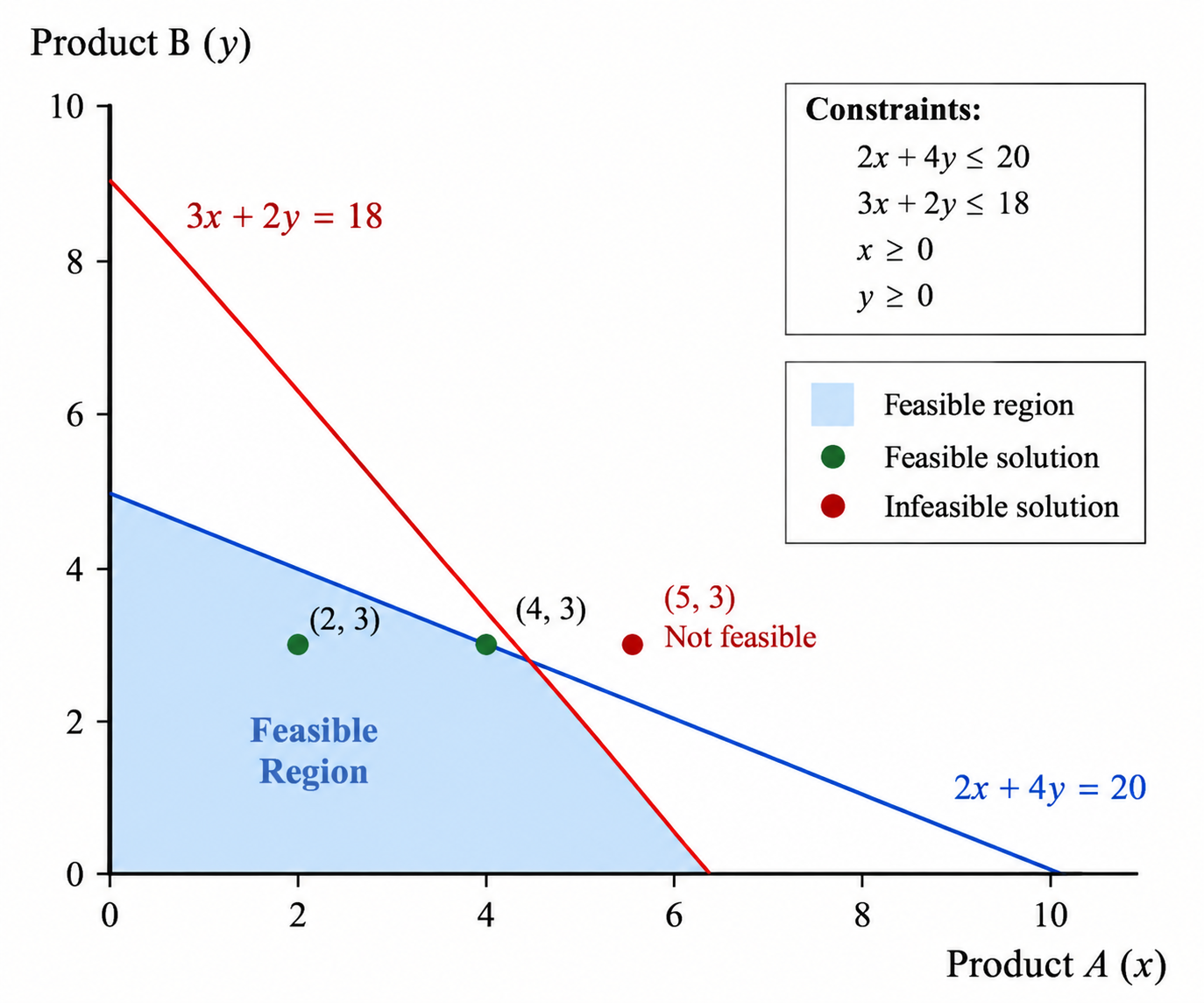
For our problem, the corner points are:
We can calculate the profit at each point using:
Check each corner point
Point 1: \((0,0)\)
Profit:
Point 2: \((6,0)\)
Profit:
Point 3: \((4,3)\)
Profit:
Point 4: \((0,5)\)
Profit:
We can summarize the results:
| \(x\) | \(y\) | Profit |
|---|---|---|
| 0 | 0 | $0 |
| 6 | 0 | $60 |
| 4 | 3 | $85 |
| 0 | 5 | $75 |
The highest profit is:
at:
Therefore, the optimal solution is:
- Produce 4 units of Product A
- Produce 3 units of Product B
- Maximum profit = $85
This demonstrates the basic manual solution process:
4. Solving Larger LP Problems
The manual approach works well for a small problem with two variables.
However, real LP problems can have:
- Hundreds or thousands of decision variables
- Many constraints
- Large numbers of possible solutions
Checking every possible solution manually is not practical.
This is where LP algorithms and solvers become useful.
An LP solver is software that takes the mathematical formulation of an LP problem and calculates the optimal solution automatically.
Conceptually:
The solver handles the mathematical search for us.
We do not need to manually calculate every possible combination of decision variables.
Common LP Algorithms
Some commonly used algorithms for solving LP problems are:
- Simplex Method
- Revised Simplex Method
- Interior-Point Methods
You do not need to learn the internal details of these algorithms for now.
The important idea is:
We formulate the optimization problem. The solver uses an algorithm to find the optimal solution.
For small problems, solving manually helps us understand what the solver is doing.
For larger problems, we normally let the solver do the computational work.
5. Solving LP with Python
Once we understand how an LP problem works manually, we can use Python to solve the same problem automatically.
For basic LP problems, SciPy provides an optimization function called linprog.
The LP problem from our example is:
Subject to:
Using scipy.optimize.linprog
One detail is important: linprog solves minimization problems by default.
Our problem is a maximization problem, so we can minimize the negative of the objective:
The Python code is:
from scipy.optimize import linprog

result = linprog(
    c=[-10, -15],
    A_ub=[
        [2, 4],
        [3, 2]
    ],
    b_ub=[20, 18],
    bounds=[
        (0, None),
        (0, None)
    ],
    method="highs"
)

print(result.x)
print(-result.fun)
The solver returns approximately:
[4. 3.]
85.0
So Python gives us:
and:
This matches the result we obtained manually.
What Did We Give the Solver?
We provided the same three building blocks we learned in Part 2:
| LP Component | Python |
|---|---|
| Decision Variables | x, y |
| Objective Function | c=[-10, -15] |
| Constraints | A_ub, b_ub |
| Variable Bounds | bounds |
The important point is that Python is not replacing the LP formulation.
We still need to understand and formulate the problem correctly.
Python and the solver simply perform the mathematical computation needed to find the solution.
6. Summary
We started with the LP problem we formulated in Part 2:
Subject to:
We then solved it manually by:
- Finding where the constraint boundaries intersect
- Checking feasible solutions
- Evaluating the objective function
- Identifying the optimal solution
The optimal solution was:
with a maximum profit of:
We then used a Python LP solver to solve the same problem automatically and obtained the same result.
The overall process is:
For small problems, we can understand the solution process manually.
For larger problems, an LP solver or Python can perform the computational work for us.